In this article, we are going to show how a symbolic regression model can be visualized using the R programming language. The model will be generated using the TuringBot symbolic regression software, and we are going to use the ggplot2 library [1] for the visualization.
The dataset that we are going to use consists of the closing prices for the S&P 500 index in the last year, downloaded from Yahoo Finance [2]. The CSV file, which also contains additional columns like open, high, low, and volume, can be found here: spx.csv
- TuringBot formulas work directly in R with standard math functions
- Modeled S&P 500 closing prices with a compact trigonometric formula
- 50/50 train/test split ensures model generalizes to unseen data
- Unlike neural networks, the formula is directly plottable in ggplot2
Symbolic regression modeling
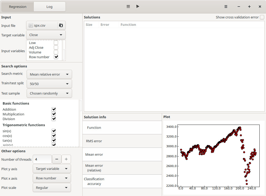
After opening TuringBot and selecting this file from the menu on the upper left of the interface, we set:
- Target variable: Close
- Input variables: just "Row number" (this way, our model will find the close price as a function of the index of the trading day)
- Search metric: Mean relative error (because we are more interested in the shape of the model than in specific values)
- Train/test split: 50/50 (we use cross-validation to make our model more robust)
- Test sample: Chosen randomly
This is what the interface will look like:
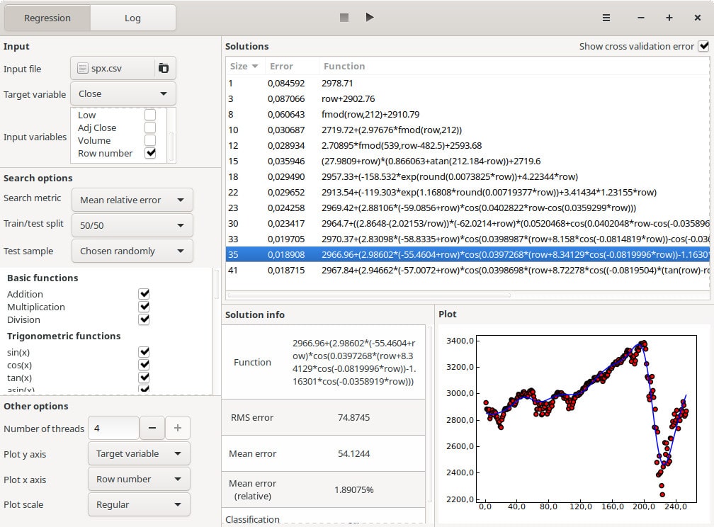
Clicking on the play button at the top, the optimization is started, using all the CPU cores in the computer for greater performance. The models encountered so far are seen in the “Solutions” box.
Selecting the best formula
After letting the optimization run for a few minutes, we can click on the “Show cross-validation error” box on the upper right of the interface to see the out-of-sample performance of each model, and use this information to select the best one, which in this case turned out to be a combination of cosines and multiplications:
Visualizing with R and ggplot2
Now that we have the model, we are going to visualize it using ggplot2. The following script loads the input CSV file and plots it along with the model that we just selected:
library(ggplot2)

# Read data from CSV file
data <- read.csv("spx.csv")
data$idx <- as.numeric(row.names(data))
print(data)

# Define the equation function
eq <- function(row) {
  2966.96 + (2.98602 * (-55.4604 + row) * cos(0.0397268 * (row + 8.34129 * cos(-0.0819996 * row)) - 1.16301 * cos(-0.0358919 * row)))
}

# Create the ggplot object
p <- ggplot(data, aes(x = idx, y = Close)) +
  geom_point() +
  stat_function(fun = eq, color = 'blue')

# Display the plot
print(p)

# Save the plot as a PNG file
# png("test.png")
# print(p)
# dev.off()
And this is the final result:
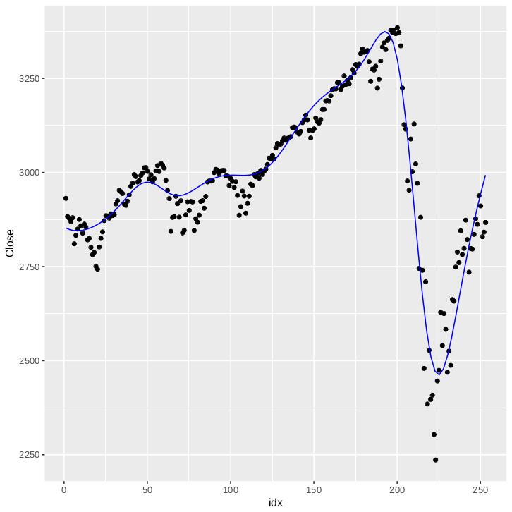
This demonstrates the power and simplicity of symbolic regression models: we have managed to readily implement and visualize a model generated using TuringBot into R, something that would be much harder if the model was a black box like a neural network or a random forest. The formula is completely transparent, interpretable, and can be embedded anywhere.
Why TuringBot for R Users?
| Feature | TuringBot | R Packages (gramEvol, rgp) |
|---|---|---|
| Installation | Standalone binary | CRAN + dependencies |
| Performance | Compiled C++, multi-threaded | Interpreted R |
| Formula export | Direct R-compatible syntax | R native |
| Cross-validation | Built-in with visual feedback | Manual setup required |
| GUI | Full visual interface | Code only |
The discovered formula uses standard R functions (cos), making it directly usable in ggplot2's stat_function() without any conversion. You can download TuringBot for free and try it with your own data.
References
[1] ggplot2: https://ggplot2.tidyverse.org/
[2] Yahoo Finance quotes for the S&P 500: https://finance.yahoo.com/quote/%5EGSPC?p=^GSPC&.tsrc=fin-srch