Load a CSV, pick the column you want predicted, and TuringBot searches for the equation: the structure of the expression and its coefficients at the same time. You do not choose the form first, and you are not limited to one input variable. It is a desktop application for Windows, macOS and Linux, and there is a free version.
Download TuringBotSee pricingSkip to the worked example
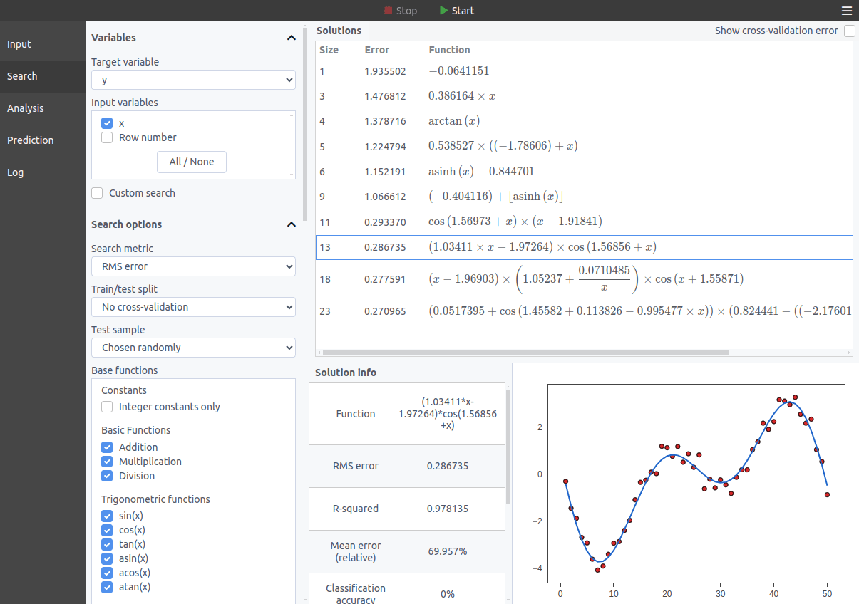
Conventional curve fitting works the other way round. You supply the model and least squares finds its coefficients.
The difference in one sentence
Classical curve fitting: you supply the form, the software finds the constants.
Symbolic regression: the software finds the form and the constants.
The better packages narrow the gap by trying a large built-in library on your behalf and ranking the results. TableCurve 2D advertises more than 3,600 built-in equations, and CurveExpert Professional handles multiple input variables and ranks its models for you. That covers a lot of ground. What none of them can return is a form that was never in the library, and for that you have to write the equation yourself.
Example: recovering an equation from two variables
This example uses synthetic data generated from a known engineering equation, so the right answer is known in advance. The Dittus-Boelter correlation is a standard result in heat transfer, found in every textbook on the subject. It relates the Nusselt number to the Reynolds and Prandtl numbers:
Nu = 0.023 * Re^0.8 * Pr^0.4We generated 50 data points from this relationship over a realistic range (Re from 10,000 to 120,000, Pr from 0.7 to 12) and added 2% random noise to imitate measurement error.
We gave TuringBot the three columns and restricted the available operations to multiplication and powers. That restriction is prior knowledge: engineering correlations of this kind are usually power laws, and an engineer fitting one would make the same choice. What we did not supply was the structure of the expression or any of its three constants. The search ran for three minutes.
This is what it returned:
Nu = pow(8.02289e-05 * Re * Pr * Re, 0.3997582)Expanding that expression gives:
Nu = 0.02305 * Re^0.7995 * Pr^0.3998Against the true values of 0.023, 0.8 and 0.4, the exponents are recovered to about 0.06% and the leading constant to within 0.23%, from 50 noisy points, without being told the shape of the expression or any of its constants.
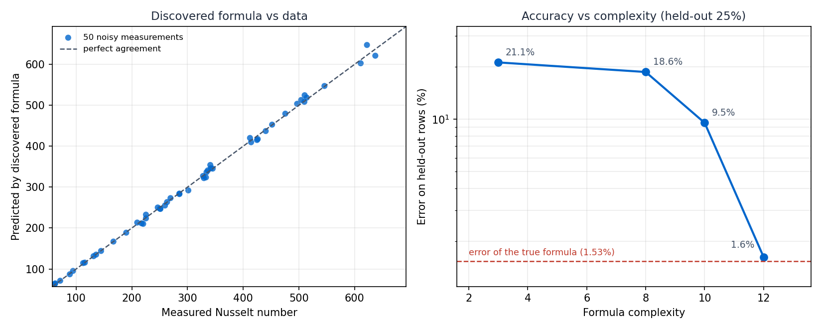
The more useful number is this one. Across all 50 rows, the discovered formula has a mean relative error of 1.495%. The true Dittus-Boelter formula, scored on the same 50 rows, gives 1.527%. The errors are close enough that the discovered formula has landed near the accuracy the noise allows. Its slightly lower figure is not evidence that it predicts new measurements better; on 50 noisy points a small gap in either direction is expected.
These two figures are measured on all 50 rows. The error column in the table below is different: it is measured only on the 25% of rows held back from the search, which is why it reads slightly higher.
You get a range of answers, not one
TuringBot does not return a single equation. It returns the best formula it found at every level of complexity, scored on data it was not trained on. For the run above:
| Complexity | Formula | Test error |
|---|---|---|
| 3 | 0.0044794 * Re | 21.1% |
| 8 | pow(Pr*Re, 0.45064) | 18.6% |
| 10 | 0.0024937*pow(Pr, 0.39077)*Re | 9.5% |
| 12 | pow(8.02289e-05*Re*Pr*Re, 0.39976) | 1.6% |
Scoring on a held-out sample is what lets you see where extra complexity stops buying accuracy. Note that this is opt-in: TuringBot defaults to no test sample, and the run above set a 75/25 split explicitly. Conventional fitting tools can be validated the same way, and some report model-selection statistics such as AIC for the same purpose. The difference is not the validation, it is that the list being compared was produced by searching over expression structures rather than drawn from a fixed library.
How it compares to classical curve fitting
| Library curve fitting | TuringBot | |
|---|---|---|
| Who chooses the equation | You, or a fixed built-in list | The search |
| Input variables | Varies by package; several support many | No fixed limit |
| Overfitting check | Ranking statistics, AIC, or your own validation | Built-in train and test split, off by default |
| Output | Best-ranked equation | One equation per complexity level |
| Export | Varies | Python, C, C++, LaTeX, plain text |
| Automation | Varies | Command line and Python library |
| Platforms | Often Windows only | Windows, macOS, Linux |
When a classical curve fitter is the better tool
Symbolic regression is not the right answer to every fitting problem, and it is worth being direct about that.
- You already know the physics. If theory tells you the relationship is a single exponential decay, fit an exponential decay. A least-squares fit of a known form is faster, gives you confidence intervals on each parameter, and is easier to defend.
- You need parameter uncertainties. Packages built around nonlinear least squares report standard errors and covariances for the fitted parameters. TuringBot returns the expression, not an uncertainty analysis of its constants.
- Peak fitting and spectroscopy. Deconvolving overlapping peaks is a specialized problem, and dedicated tools handle it better.
- Very small datasets. With a handful of points, a search over expressions has too much freedom. Choose a form and fit it.
Symbolic regression earns its place when you genuinely do not know the form, when there are several interacting inputs, or when you need a compact equation you can put in a report, embed in firmware, or hand to a colleague who will ask how it works.
Running it
Load a CSV or TXT file with one variable per column, choose which column to predict, and start the search. The last column is the target by default. Results appear within seconds and keep improving while the search runs.
The same search runs from the command line, with every option available as a flag:
turingbot heat.txt \
  --search-metric 1 \
  --train-test-split 75 \
  --allowed-functions "* pow" \
  --threads 24 \
  --outfile results.txt
Or from Python, which takes a NumPy array or a pandas DataFrame directly, so you do not have to write an input file yourself:
import time
import turingbot as tb

sim = tb.simulation()
sim.start_process(
    input_file=data,                  # NumPy array or DataFrame
    column_names=["Re", "Pr", "Nu"],
    search_metric=1,                  # mean relative error
    train_test_split=75,
    maximum_formula_complexity=14,
    allowed_functions="* pow",
    threads=24,
)

time.sleep(180)                       # the search runs in the background
sim.refresh_functions()
print(*sim.functions, sep="\n")
sim.terminate_process()
Download TuringBot for Windows, macOS or Linux to get the application itself. The Python library drives that installed application, so add pip install turingbot if you want to automate it. The documentation lists every option, error metric and base function, and pricing covers the license options.
If your problem is really a classical fitting problem, where you already know the form and need good parameter estimates, the curve fitting software comparison covers the alternatives, several of which are free.
Reproducing the example
The dataset is 50 rows of Re, Pr and Nu generated from the Dittus-Boelter relationship with 2% multiplicative Gaussian noise. The search used multiplication and powers as its operators, a maximum formula complexity of 14 (the default is 60) and a 75/25 train and test split with seed 42. Both files are here so you can check the result rather than take our word for it:
- heat.txt, the input dataset (50 rows, so it runs on the free version)
- results.txt, the unedited output of the command below
This is the exact command, run with TuringBot 3.3.1:
turingbot heat.txt \
  --search-metric 1 \
  --train-test-split 75 \
  --train-test-seed 42 \
  --maximum-formula-complexity 14 \
  --allowed-functions "* pow" \
  --threads 24 \
  --outfile results.txt
It ran for three minutes on 24 threads. The expanded form shown earlier is an algebraic rewrite of the expression TuringBot returned, not a separate result. Simulated annealing is stochastic, so a rerun will not reproduce the constants digit for digit, and a shorter run on fewer threads will explore less.
For contrast, an earlier run with the default, unrestricted function set did not recover the power law. It reached 2.0% test error using a sqrt(Pr) term instead, which is close to the noise floor but not the textbook form. Narrowing the function set to what the physics suggests is what made the difference.