Introduction
TuringBot, named after the great mathematician and computation pioneer Alan Turing, is a desktop software for Symbolic Regression. It uses a novel algorithm based on simulated annealing to discover mathematical formulas from numerical values with unprecedented efficiency.
You can enter data through the built-in spreadsheet or by importing CSV or TXT files. The target and input columns can be selected in the interface. A variety of error metrics are available for the search, allowing the program to find formulas that solve both regression and classification problems.
The main features of TuringBot are the following:
- Pareto optimization: the software simultaneously tries to find the best formulas of all possible sizes. It gives you not only a single formula as output but a set of formulas of increasing complexity to choose from.
- Built-in train/test split: allows you to easily rule out overfit solutions.
- Export solutions as Python, C/C++, LaTeX, or plain text.
- Multiprocessing.
- Written in a low-level programming language, making it extremely fast.
- Make numerical predictions from the generated models directly through the UI.
- Has a command-line mode that allows you to automate the program.
Data input
To enter data into the program, use the Input tab (see below). There, you can paste data copied from any spreadsheet program, and you can also import data from an existing file:
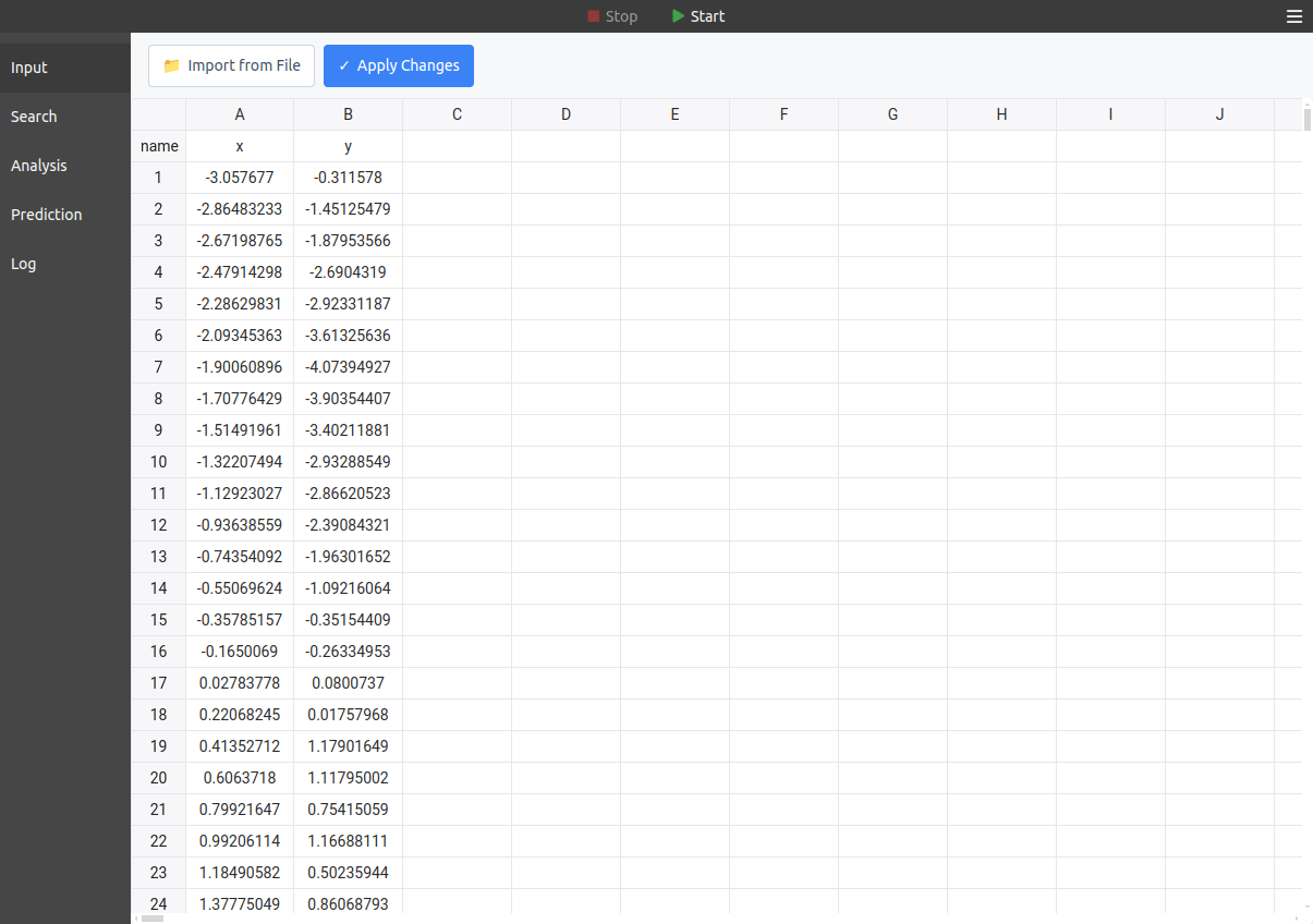
After pasting data manually, it's necessary to click on the "Apply Changes" button to load it.
Importing files
To import data, your file must have a .txt or .csv extension, and it must contain data columns separated by spaces, commas, semicolons, or tabs. These values can be integers, floats, or floats in exponential notation (%d, %f, or %e), with decimal parts separated by a dot (1.61803 and not 1,61803).
Optionally, a header containing the variable names may be present in the first line of the file — in this case, those names will be used in the formulas instead of the default names, which are col1, col2, col3, etc.
For example, the following is a valid input file:
x,y,z
0.01231,0.99992,0.99985
0.23180,0.97325,0.94723
0.45128,0.89989,0.80980
0.67077,0.78334,0.61363
0.89026,0.62921,0.39591
1.00000,0.54030,0.29193
The following elements must not be present in the input file:
- Text or string data (except in the header).
- Date values (e.g., 2024-09-15 or 09/15/2024).
- Currency symbols (e.g., $).
- Percentage symbols (e.g., %).
- Commas in numeric values (e.g., 6,000.00 should be 6000.00).
- Parentheses around numbers (e.g., (100)).
- Spaces in header names (use underscores instead: variable_name).
If any of the above elements are present, the program will fail to parse the file correctly.
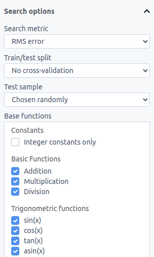
Search options
On the left side of the Search tab, you can set a variety of search settings, including the error metric and the base functions that should be used in the optimization:
Error metrics
The available error metrics are:
| Metric | Description |
|---|---|
| RMS error | Root mean square error. |
| Mean error | Average of (absolute value of the error). Similar to RMS error, but it puts less emphasis on outliers. |
| Percentile error | Returns the specified percentile of all absolute errors. Takes a parameter between 0 and 1, where 0.5 gives the median absolute error, and 1.0 gives the maximum absolute error |
| Maximum error | The maximum absolute difference between the predictions of the model and the target variable. |
| Mean relative error | Average of (absolute value of the error) / (absolute value of the target variable). With that, the convergence is in terms of relative error instead of absolute error. When the target variable is zero, the absolute error is used instead. |
| Maximum relative error | The maximum of (absolute value of the error) / (absolute value of the target variable). |
| Correlation coefficient | Corresponds to the Pearson correlation coefficient. Useful for quickly getting the overall shape of the output right without attention to scales. |
| Hybrid (CC+RMS) | The geometric mean between the correlation coefficient and the RMS error. This is a compromise between the attention to scale of the RMS metric and the speed of the CC metric. |
| Nash-Sutcliffe efficiency | A metric that resembles the correlation coefficient and is commonly used in hydrological applications. See the definition in this paper. |
| Residual sum of squares (RSS) | The sum of (predicted - observed)^2. Very similar to the RMS metric but without taking the average and the square root. |
| Root mean squared log error (RMSLE) | The square root of the average of (log(1 + predicted) - log(1 + observed))^2. Like mean relative error, this metric can be applied to target variables that span multiple orders of magnitude, but it penalizes large errors less aggressively, and is thus less sensitive to outliers. It requires the target variable to be non-negative (>= 0). |
| Classification accuracy | (correct predictions) / (number of data points). Only useful for integer target values and classification problems. |
| F-score | 2*(precision*recall)/(precision+recall) when "F-score beta parameter" is set to 1. See here an image that explains what those two quantities are. This metric is useful for classification problems on highly imbalanced datasets, where the target variable is 0 for the majority of inputs and a positive integer for a few cases that need to be identified. If the classification is binary, then the categories can be 1 (relevant cases) and 0 (all other cases). For multiclass problems, predictions must match the exact class value to be considered correct. |
| Binary cross-entropy | Used for solving binary classification problems in terms of probabilities. To use this metric, your target variable must contain two (and only two) classes represented by the numbers 0 and 1. |
| Matthews correlation coefficient | A classification metric that takes into account true positives, true negatives, false positives, and false negatives and can be used even if the categories have imbalanced numbers of elements. To use this metric, your "negative" target variable must be represented by the number 0, and your "positive" variables must be represented by one or more positive integer numbers. Predictions must match the exact class value to be considered correct (e.g., predicting 2 when the actual class is 1 counts as a false positive). See this paper for details. |
| Custom metric | A user-defined error metric formula. See the Custom metric section below for details. |
Custom metric
TuringBot allows you to define a custom error metric using a formula. This gives you full control over how the search evaluates candidate solutions. In the UI, select "Custom metric" from the "Search metric" dropdown in the Search tab — a text field will appear where you can enter your formula.
In your formula, you can use aggregation functions that operate on per-row values:
- sum() — sum over all data points
- mean() — average over all data points
- median() — median over all data points
- maxval() — maximum over all data points
- minval() — minimum over all data points
Inside these aggregation functions, you can use the per-row variables actual (the target value) and predicted (the model's prediction). These two variables must appear inside an aggregation function.
You can also use the following built-in metric scalars directly in your formula (outside aggregation functions):
- rms — RMS error
- mae — Mean error
- mre — Mean relative error
- maxerr — Maximum error
- maxre — Maximum relative error
- accuracy — Classification accuracy
- correlation — Correlation coefficient
- nash — Nash-Sutcliffe efficiency
- logloss — Binary cross-entropy
- mcc_val — Matthews correlation coefficient
- rss — Residual sum of squares (RSS)
- rmsle — Root mean squared log error (RMSLE)
The variable n represents the number of data points. Standard math functions (such as pow, sqrt, abs, log, exp, etc.) are also available.
Examples:
- Mean squared error: mean(pow(actual-predicted,2))
- Root mean squared error: sqrt(mean(pow(actual-predicted,2)))
- Maximum absolute error: maxval(abs(actual-predicted))
- Weighted combination: 0.5*rms+0.5*mae
- Sum of squared errors divided by n: sum(pow(actual-predicted,2))/n
Base functions
The function names follow the conventions of the C math library. You can find their definitions on this page.
The exceptions are the logical functions (logical_and(x, y), greater(x, y), etc), the history functions (delay, moving_average, and decay), and sign (the sign function), which are defined internally in TuringBot.
The default sizes of the base functions are defined as:
- Size 1: an input variable, sum, subtraction, multiplication, and mathematical constants.
- Size 2: division.
- Size 3: abs(x), ceil(x), floor(x), and round(x).
- Size 4: all other functions.
These sizes are customizable. In the UI, you can adjust the size of each function using the number inputs next to each function checkbox. From the command line, use the --function-size flag with space-separated name:size pairs, for example --function-size "sin:3 cos:3 pow:5". Only overrides need to be specified; unspecified functions keep their defaults.
Mathematical constants can optionally be included in the search:
- pi - π (approximately 3.14159)
- e - Euler's number (approximately 2.71828)
- sqrt2 - Square root of 2 (approximately 1.41421)
- ln2 - Natural logarithm of 2 (approximately 0.69315)
- gamma - Euler-Mascheroni constant (approximately 0.57722)
- phi - Golden ratio (approximately 1.61803)
The moving average of a variable is defined as its average value in the N rows before the present one. For instance, if the successive values for variable x are (1, 2, 3, 4, 5), then at x = 5, the value for moving_average(x,3) will be (2+3+4)/3. In some systems, this may be considered a moving average with a lag of 1.
The decay function decay(x, r) computes an exponentially weighted sum of past values: f(t) + r*f(t-1) + r^2*f(t-2) + ..., where 0 < r < 1. This gives more weight to recent values and exponentially decreasing weight to older ones.
Custom functions
In the "Custom functions" text field at the bottom of the base functions list you can define your own unary or binary base functions. These will be used in the search alongside the built-in ones.
- Unary functions are defined as name(x)=expr
- Binary functions are defined as name(x,y)=expr
The default complexity for these functions is 4. You can optionally specify a custom complexity cost using the |cost suffix. For example, gauss(x)=exp(-x*x)|2 defines a function with complexity 2.
Custom functions can reference previously defined custom functions.
Examples:
- bump(x)=exp(-x*x) — unary, default complexity 4
- mydist(x,y)=sqrt(x*x+y*y) — binary
- gauss(x)=exp(-x*x)|2 — unary with complexity 2
- double(x)=x+x,quadruple(x)=double(double(x)) — chaining: quadruple references double
Custom constants
In the "Custom constants" text field at the bottom of the base functions list, just above "Custom functions", you can define custom constants for the search. These are treated like the built-in mathematical constants but with user-specified values.
Each constant is defined in the format name=value. You can optionally specify a custom complexity cost using the |cost suffix.
Examples:
- g=9.81,c=299792458 — two constants with default complexity 1
- sun=1.989e30|7 — one constant with complexity 7
Custom search
By default, the program finds formulas in the form y = f(x1,x2,x3,...). However, you may want to search for specific functional forms. Here are some examples:
- A line: y = f()*x + f()
- A parabola: y = f()*x*x + f()*x + f()
- A formula with terms that depend on specific variables: y = f(x1,x2)*x1 + exp(f(x1)/4) + 2
You can perform this kind of search using TuringBot's custom search mode. To enable it, check the "Custom search" checkbox and enter your desired equation in the input box that appears:
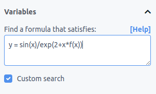
The left side should contain your target variable, and the right side should contain the formula you want to find, with unknown terms written as f(variable1,variable2,...).
When writing your custom equation, follow these rules:
- Write unknown terms as f(variable1,variable2,...). For a constant, use f(). For a function of x, use f(x). For a function of x and z, use f(x,z). And so on.
- To create a function of all variables except one, use the ~ operator. For example, f(~y) will use all variables except y, and f(~y,~row) will use all variables except y and row.
- Constants must be written as integers, floating-point numbers, or in exponential notation (like 2, 3.14, or 2.35e-3).
-
To use an unknown term multiple times in your equation, write it as an indexed term by adding a number after f. For example:
y = f1() + f1()*x
Both instances of f1() will be identical, creating a line with the same intercept and slope. Similarly, in:
y = f1(x) / (1 + f1(x))
Both occurrences of f1(x) will represent the same function. You can use different indexed functions as needed:
y = f1(x) + f1(x) + f2() / (1 + f2())
Here, the two f1(x) terms are identical, and the two f2() terms are identical.
You can use any of the program's base functions in your custom equation. During custom search, the plot will display the left side of the equation as points and the right side as a line.
Custom input expressions
You can pass expressions as extra inputs to f() terms. For example, y = f(x, x*x) lets the search use both x and x*x as inputs.
Each custom input expression has a complexity of 1, just like a regular variable, regardless of its size. Expressions can use any base function, built-in or custom constant, or custom function.
Examples:
- y = f(x, exp(-x)) — the search can use both x and exp(-x)
- y = f(x, 3*x+1, x/2, sin(x)*sin(x)) — multiple derived inputs
Train/test split
Below the "Search metric" dropdown, you can find the test sample settings. It is recommended to use test sample since that allows overfit models that are more complex than necessary to be discarded in a straightforward way.
The size of the train/test split can be selected from the "Train/test split" menu. The default value, "No test sample", disables the test sample altogether. Three kinds of options are available:
- Percentages like 50/50 and 80/20.
- Fixed training dataset sizes like "100 rows" and "1000 rows".
- A "Custom rows" option where you can specify the exact number of rows for the training set.
It is also possible to select how the training sample should be generated: if it should be a selection of random rows or the first rows in your dataset in sequential order.
During the optimization, you can alternate between showing the errors for the training sample and the testing sample by clicking on the "Show test sample error" box on the upper right of the interface. With this, overfit solutions can be spotted in real time.
Other options
Under "Advanced search options", the following additional settings can be found:
| Parameter | Description |
|---|---|
| Maximum formula size | By default, the complexity of formulas is prevented from becoming larger than 60. With this option, you can allow the program to generate larger formulas, which makes the optimization slower but makes longer formulas possible. |
| Maximum history size | Only used if one of the history functions is enabled. Sets the maximum length of those functions. Note that if this parameter is set to 20, then the first 20 rows of your dataset are not used for the search, and are only used to calculate the history functions starting from row 21. |
| Maximum occurrences per variable | Limits how many times a single variable can appear in a formula. This helps control formula complexity and prevents over-reliance on individual variables. |
| Number of distinct variables | Sets the minimum and maximum number of different variables that can be used in a single formula. Allows you to control the complexity and interpretability of solutions. Default is -1 (unset) for both values; you can set just the minimum or maximum by leaving the other at -1. |
| Number of constants | Sets the minimum and maximum number of numerical constants that can be included in a formula. Default is -1 (unset) for both values; you can set just the minimum or maximum by leaving the other at -1. |
| CPU threads | The number of CPU threads to use. It defaults to the maximum for your CPU. |
| Bound search mode | This advanced search mode allows you to discover formulas that are upper or lower bounds for the target variable. |
| Normalize the dataset | For each variable, subtract the average and divide by the standard deviation before starting the search. This can speed up the search a lot if your input variables are large. Note that the "sample standard deviation" is used, where the denominator is N-1 instead of N for smaller bias: link. In the output formulas, you will see (var-avg)/std instead of var for each variable when this option is checked. |
| Target variable in history functions | Allows you to choose whether your target variable can be used in the history functions. |
| Force solutions to include all variables | Allows you to discard solutions that do not feature all input variables. |
| Random seed for train/test split generation | If a value >= 0 is set, this value will be used as a seed, resulting in the same split every time a new search is started with the same dataset. When the parameter is set to -1, a different random split will be generated each time. |
| F-score beta parameter | When left at the default value of 1, the F-score metric corresponds to the F1-metric. Values of beta lower than 1 favor precision over recall. |
The solutions box
The regression is started by clicking on the play button at the top of the interface. After that, the best solutions found so far will be shown in the "Solutions" box, as shown below:
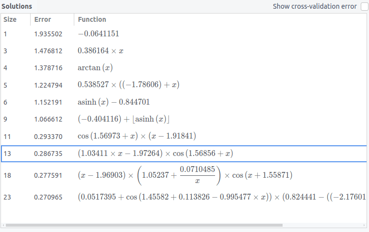
Each row corresponds to the best solution of a given size encountered so far. By clicking on a solution, it will be shown in the plot and its stats will be shown in the "Solution info" box. Larger solutions are only shown if they provide a better fit than all smaller solutions.
The size of a solution is defined as the sum of the sizes of the base functions that constitute it (see above).
In the Solutions box, you have the option of sorting the solutions by a balance between size and accuracy by clicking on the "Function" header, which will sort the solutions by (error)^2 * (size). By default, the solutions are sorted by size.
Plot settings
Under "Plot options", you can change your plot settings at any time:
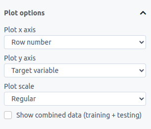
In the "Plot type" dropdown, you can choose between Regular for standard plotting or Observed vs predicted to see how well your solutions match the target data. The observed vs predicted plot also shows a gray line representing a perfect fit for visual reference.
For the y-axis, you can choose to plot your target variable, the residual error (difference between a solution and the target data), and the residual error as a percentage of the target data.
For the x-axis, you can choose the row number (1, 2, 3, ...) corresponding to that point, or any of your input variables.
The plot scales can be adjusted in the "Plot scale" menu, where you can choose from regular scale, log x, log y, or log x and y. The "log" scale uses the regular base 10 logarithm.
If test sample is enabled, you can optionally view the full dataset in the plot by clicking on "Show combined data (training + testing)".
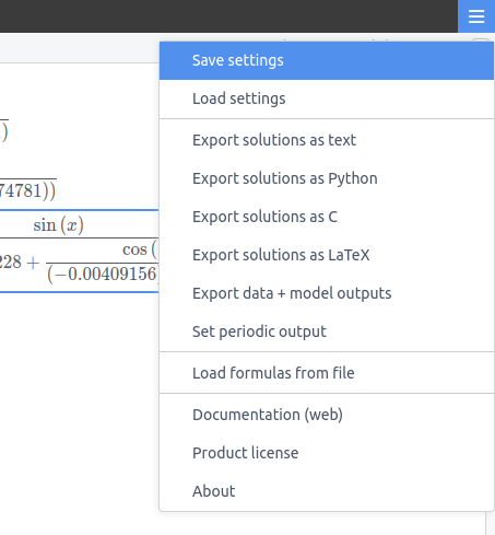
Exporting/loading formulas
You can export the current solutions using "Export solutions as text" from the menu. This creates a solutions.txt file containing all discovered formulas. This exported file can then be loaded back into the program using "Load formulas from file" in the menu, allowing you to:
- Resume an optimization from a checkpoint
- Transfer solutions between different datasets or search configurations
- Combine results from multiple search runs
You can select and load multiple solutions.txt files simultaneously, and the formulas will work even if you change the search metric or other settings between export and import.
You can also create custom formula files manually by writing one formula per line in a text file and loading it using the same "Load formulas from file" option. The formulas should use your dataset's variable names and any of the available base functions.
For automated workflows, "Set periodic output" in the menu can automatically export the same solutions.txt file at regular intervals, but only when new solutions are found. The periodic output also offers a "Predictions" option that exports your original dataset along with model predictions, where prediction columns are named solution_N (N being the formula complexity).
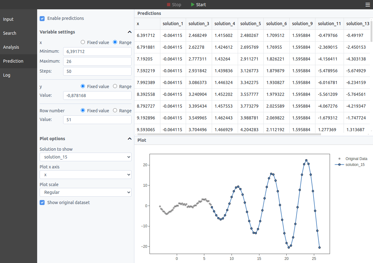
Making predictions
In the Predictions tab, you can calculate the outputs for the current models with custom inputs. For each variable, you can choose between setting a fixed value and setting a range of values. In the latter case, a plot will be shown with the varying variable in the x axis; if more than one varying variable is available, you can choose which one to show in the plot in the "Plot x axis" dropdown.
The predictions are recalculated in real time as new solutions emerge during the search.
Running TuringBot from Python
The TuringBot Python library can be installed with:
pip install turingbot
After updating TuringBot, run pip install -U turingbot to keep the library in sync.
The library provides a simulation class:
sim = tb.simulation()
This class has a start_process method that starts TuringBot in the background:
start_process(
    path: str = None,
    input_file=None,
    config: str = None,
    column_names: list = None,
    threads: int = None,
    outfile: str = None,
    predictions_file: str = None,
    formulas_file: str = None,
    search_metric: int = None,
    train_test_split: int = None,
    test_sample: int = None,
    train_test_seed: int = None,
    bound_search_mode: int = None,
    maximum_formula_complexity: int = None,
    history_size: int = None,
    max_occurrences_per_variable: int = None,
    distinct_variables_min: int = None,
    distinct_variables_max: int = None,
    constants_min: int = None,
    constants_max: int = None,
    fscore_beta: float = None,
    percentile: float = None,
    integer_constants: bool = False,
    normalize_dataset: bool = False,
    allow_target_delay: bool = False,
    force_all_variables: bool = False,
    custom_formula: str = None,
    custom_constants: str = None,
    custom_functions: str = None,
    custom_metric: str = None,
    allowed_functions=None,
    function_size: str = None,
)
    Start the process with the specified configuration and dataset.

    Parameters:
    -----------
    path : str, optional
        Path to the TuringBot executable. If not provided, the default
        installation path for your OS will be used automatically.
    input_file : str, numpy.ndarray, or pandas.DataFrame
        The input data. Can be a file path (str), a 2D numpy array,
        or a pandas DataFrame. When an array or DataFrame is passed,
        it is saved to a temporary CSV file automatically.
    config : str, optional
        Path to the configuration file.
    column_names : list of str, optional
        Column names for the data. Only used when input_file is a
        numpy array. Ignored for DataFrames (which have their own
        column names) and file paths.
    threads : int, optional
        Number of threads to use.
    outfile : str, optional
        Output file path.
    predictions_file : str, optional
        File to store predictions.
    formulas_file : str, optional
        File to store generated formulas.
    search_metric : int, optional
        Search metric to use. Default is 4 (RMS error).
        Options:
        1: Mean relative error
        2: Classification accuracy
        3: Mean error
        4: RMS error (default)
        5: F-score
        6: Correlation coefficient
        7: Hybrid (CC + RMS)
        8: Maximum error
        9: Maximum relative error
        10: Nash-Sutcliffe efficiency
        11: Binary cross-entropy
        12: Matthews correlation coefficient (MCC)
        13: Residual sum of squares (RSS)
        14: Root mean squared log error (RMSLE)
        15: Percentile error
        16: Custom metric (requires custom_metric parameter)
    train_test_split : int, optional
        Train/test split. Default is -1 (no test sample).
        Options:
        -1: No test sample (default)
        50, 60, 70, 75, 80: Percentage split for training data
        100, 1000, 10000: Predefined row counts for training
        Negative values (e.g., -200): Use 200 rows for training
    test_sample : int, optional
        How to select test samples. Default is 1 (random).
        Options:
        1: Chosen randomly (default)
        2: The last points
    train_test_seed : int, optional
        Random seed for train/test split generation. Default is -1 (no specific seed).
    bound_search_mode : int, optional
        Whether to use bound search mode. Default is 0 (deactivated).
        Options:
        0: Deactivated (default)
        1: Upper bound search
        2: Lower bound search
    maximum_formula_complexity : int, optional
        Maximum formula complexity. Default is 60.
    history_size : int, optional
        History size for the optimization process. Default is 20.
    max_occurrences_per_variable : int, optional
        Maximum occurrences per variable. Default is -1 (no limit).
    distinct_variables_min : int, optional
        Minimum number of distinct variables. Default is -1 (no limit).
    distinct_variables_max : int, optional
        Maximum number of distinct variables. Default is -1 (no limit).
    constants_min : int, optional
        Minimum number of constants. Default is -1 (no limit).
    constants_max : int, optional
        Maximum number of constants. Default is -1 (no limit).
    fscore_beta : float, optional
        Beta parameter for F-score. Default is 1.
    percentile : float, optional
        Percentile for the Percentile error metric. Default is 0.5.
    integer_constants : bool, optional
        Whether to use integer constants only. Default is False (disabled).
    normalize_dataset : bool, optional
        Whether to normalize the dataset before optimization. Default is False (no normalization).
    allow_target_delay : bool, optional
        Whether to allow the target variable in lag functions. Default is False (not allowed).
    force_all_variables : bool, optional
        Whether to force the solution to include all input variables. Default is False (not forced).
    custom_formula : str, optional
        Custom formula for the search. If not provided, the last column will be treated as the target variable.
    custom_constants : str, optional
        Custom constants, comma-separated name=value pairs. Add |cost
        after the value to set complexity (default: 1). Examples:
          "k=1.380649e-23,h=6.62607e-34"
          "sun=1.989e30|7" (complexity 7)
    custom_functions : str, optional
        Custom base functions, comma-separated. One argument = unary,
        two = binary. Add |cost after the expression to set complexity
        (default: 4). Examples:
          "bump(x)=exp(-x*x)"
          "mydist(x,y)=sqrt(x*x+y*y)"
          "gauss(x)=exp(-x*x)|2" (complexity 2)
    custom_metric : str, optional
        Custom search metric formula. Automatically sets search_metric
        to 16.
        'actual' and 'predicted' give per-row values and must be
        inside sum(), mean(), median(), maxval(), or minval():
          "mean(pow(actual-predicted,2))"
          "sqrt(mean(pow(actual-predicted,2)))"
          "maxval(abs(actual-predicted))"
        Built-in metrics (rms, mae, mre, maxerr, maxre, accuracy,
        correlation, nash, logloss, mcc_val, rss, rmsle, n) can
        be used directly:
          "0.5*rms+0.5*mae"
    allowed_functions : str or list of str, optional
        Allowed functions for the formula search, as a list of strings
        (e.g. ["+", "sin", "cos"]) or a single string (e.g. "+ sin cos").
        Default: all functions.
    function_size : str, optional
        Override size of base functions. Format: space-separated
        name:size pairs. Only overrides need to be specified; unspecified
        functions keep their defaults. Example: "sin:3 cos:3 pow:5 /:3"
Once a simulation is started, the simulation object provides the following methods and properties:
- sim.refresh_functions() — refresh the current formulas from the running process
- sim.functions — a list of the best formulas found so far (call refresh_functions() first). Each entry is [size, error, formula], or [size, train_error, test_error, formula] when a train/test split is enabled.
- sim.info — general information about the number of formulas tried so far and any error messages
- sim.terminate_process() — stop the search and kill the TuringBot process
Example
import time
import turingbot as tb

# Initialize the simulation
sim = tb.simulation()

# Start the process with specified parameters
sim.start_process(
    input_file='input.txt',
    allowed_functions=["+", "*", "/", "pow", "sin", "cos", "exp", "log", "sqrt"],
    custom_functions="sigmoid(x)=1/(1+exp(-x)),norm(x,y)=sqrt(x*x+y*y)",
    custom_metric="sqrt(mean(pow(actual-predicted,2)))",
)

# Allow some time for the process to generate results
time.sleep(30)

# Fetch and display generated functions and simulation information
sim.refresh_functions()
print("\nGenerated Functions:")
print(*sim.functions, sep='\n')

print("\nSimulation Info:")
print(sim.info)

# Terminate the simulation process
sim.terminate_process()
The input_file parameter accepts relative or absolute paths. Typical absolute paths per OS:
- Windows: r'C:\Users\YourUsername\Desktop\input.txt'
- macOS: '/Users/YourUsername/Desktop/input.txt'
- Linux: '/home/user/input.txt'
Using NumPy arrays and DataFrames
Instead of a file path, you can pass a NumPy array or a pandas DataFrame directly to input_file.
With a NumPy array (use column_names to name the variables):
import time
import numpy as np
import turingbot as tb

x = np.linspace(0, 10, 100)
y = np.random.randn(100)
z = np.sin(x) + 0.5 * y

data = np.column_stack([x, y, z])

sim = tb.simulation()
sim.start_process(
    input_file=data,
    column_names=["x", "y", "z"],
    custom_formula="z = f(x, y)",
    search_metric=4,
)

time.sleep(10)
sim.refresh_functions()
print(*sim.functions, sep='\n')
sim.terminate_process()
With a pandas DataFrame (column names are used automatically):
import time
import numpy as np
import pandas as pd
import turingbot as tb

x = np.linspace(0, 10, 100)
y = np.random.randn(100)

df = pd.DataFrame({
    "x": x,
    "y": y,
    "z": np.sin(x) + 0.5 * y,
})

sim = tb.simulation()
sim.start_process(
    input_file=df,
    custom_formula="z = f(x, y)",
    search_metric=4,
)

time.sleep(10)
sim.refresh_functions()
print(*sim.functions, sep='\n')
sim.terminate_process()
Command-line usage
TuringBot is also a console application that can be executed in a fully automated and customizable way. The general usage is the following:
TuringBot - Symbolic Regression Software

Usage: turingbot [--help] [--version] INPUT_FILE [SETTINGS_FILE]
                 [--outfile FILENAME]
                 [--predictions-file FILENAME]
                 [--formulas-file FILENAME]
                 [--threads N]
                 [--search-metric VALUE]
                 [--train-test-split VALUE]
                 [--test-sample VALUE]
                 [--train-test-seed VALUE]
                 [--bound-search-mode VALUE]
                 [--maximum-formula-complexity VALUE]
                 [--history-size VALUE]
                 [--max-occurrences-per-variable VALUE]
                 [--distinct-variables-min VALUE]
                 [--distinct-variables-max VALUE]
                 [--constants-min VALUE]
                 [--constants-max VALUE]
                 [--fscore-beta VALUE]
                 [--percentile VALUE]
                 [--integer-constants]
                 [--normalize-dataset]
                 [--allow-target-delay]
                 [--force-all-variables]
                 [--custom-formula STRING]
                 [--custom-constants STRING]
                 [--custom-functions STRING]
                 [--custom-metric STRING]
                 [--allowed-functions STRING]
                 [--function-size STRING]

License management (headless):
       turingbot --activate KEY [--name NAME]
       turingbot --deactivate
       turingbot --license-status

Required arguments:
  INPUT_FILE                    Path to your input file.

Optional arguments:
  SETTINGS_FILE                 Path to the settings file to use
                                for this optimization.
  --help                        Show this help message.
  --outfile FILENAME            Write the best formulas found so far
                                to this file.
  --predictions-file FILENAME   Write the predictions obtained from the best
                                formulas found so far to this file.
  --formulas-file FILENAME      Load seed formulas from this file.
                                The file generated by --outfile can be
                                later used as input here.
  --threads N                   Use this number of threads. The default is
                                the total number available in your system.
  --search-metric VALUE         Specify the search metric to use:
                                1: Mean relative error
                                2: Classification accuracy
                                3: Mean error
                                4: RMS error (default)
                                5: F-score
                                6: Correlation coefficient
                                7: Hybrid (CC + RMS)
                                8: Maximum error
                                9: Maximum relative error
                                10: Nash-Sutcliffe efficiency
                                11: Binary cross-entropy
                                12: Matthews correlation coefficient (MCC)
                                13: Residual sum of squares (RSS)
                                14: Root mean squared log error (RMSLE)
                                15: Percentile error
                                16: Custom metric (use with --custom-metric)
  --train-test-split VALUE      Set the train-test split ratio:
                                -1: No test sample (default)
                                50, 60, 70, 75, 80: Percentages
                                100, 1000, 10000, 100000: Predefined row counts
                                Negative numbers: Custom row count (e.g., -200 for 200 rows)
  --test-sample VALUE           Specify the test sample selection method:
                                1: Chosen randomly (default)
                                2: The last points
  --train-test-seed VALUE       Set the seed for train-test split (-1 for random).
  --bound-search-mode VALUE     Set the bound search mode:
                                0: Deactivated (default)
                                1: Upper bound search
                                2: Lower bound search
  --maximum-formula-complexity VALUE
                                Set the maximum formula complexity (default: 60).
  --history-size VALUE          Specify the history size (default: 20).
  --max-occurrences-per-variable VALUE
                                Set the maximum occurrences per variable (-1 for no limit).
  --distinct-variables-min VALUE
                                Set the minimum number of distinct variables (-1 for no limit).
  --distinct-variables-max VALUE
                                Set the maximum number of distinct variables (-1 for no limit).
  --constants-min VALUE         Set the minimum number of constants (-1 for no limit).
  --constants-max VALUE         Set the maximum number of constants (-1 for no limit).
  --fscore-beta VALUE           Set the F-score beta value (default: 1).
  --percentile VALUE            Set the percentile for the Percentile error metric (0 to 1, default: 0.5).
  --integer-constants           Force all numerical constants to be integers.
  --normalize-dataset           Normalize the dataset before optimization.
  --allow-target-delay          Allow the target variable in lag functions.
  --force-all-variables         Force solutions to include all input variables.
  --custom-formula STRING       Provide a custom formula for the search.
                                Supports expression arguments that are
                                pre-computed as extra input columns.
                                  "y = f(x, cosh(x*y)+2)"
  --custom-constants STRING     Comma-separated name=value pairs. Append |N
                                to set complexity (default 1).
                                  "k=1.38e-23,h=6.63e-34"
                                  "sun=1.99e30|7" (complexity 7)
  --custom-functions STRING     Comma-separated definitions (one arg = unary,
                                two = binary). Append |N for complexity (default 4).
                                  "bump(x)=exp(-x*x),dist(x,y)=sqrt(x*x+y*y)"
  --custom-metric STRING        Custom metric formula (sets --search-metric 16).
                                Wrap actual/predicted in sum(), mean(), median(),
                                maxval(), or minval(). Built-in names like rms,
                                mae, correlation can be combined directly.
                                  "mean(pow(actual-predicted,2))"
                                  "0.5*rms+0.5*mae"
  --allowed-functions STRING    Specify allowed functions (default: "+ * / pow
                                fmod sin cos tan asin acos atan exp log log2
                                log10 sqrt sinh cosh tanh asinh acosh atanh
                                abs floor ceil round sign tgamma lgamma erf").
  --function-size STRING        Override size of base functions.
                                Format: space-separated name:size pairs.
                                Example: "sin:3 cos:3 pow:5 /:3"
                                Only overrides need to be specified;
                                unspecified functions keep their defaults.
If no configuration file is provided, the program will use the last column in the input file as the target variable and all other columns as input variables.
The best formulas found so far will be written to the terminal every 1 second. If you set an output file with the --outfile option, those formulas will also be regularly saved to the output file.
Note that to run the command above on Windows you have to first cd to the installation directory and then run with .\TuringBot.exe:
cd C:\Program Files (x86)\TuringBot
.\TuringBot.exe INPUT_FILE
Examples
Windows:
cd "C:\Program Files (x86)\TuringBot"
.\TuringBot.exe "C:\Users\YourName\Documents\climate_research\temperature_data.txt" \
   --outfile solutions.txt \
   --threads 8 \
   --search-metric 7 \
   --train-test-split 80 \
   --custom-formula "avg_temp = f(solar_radiation, humidity, wind_speed)" \
   --allowed-functions "+ * / pow sin cos exp log sqrt"
macOS:
/Applications/TuringBot.app/Contents/MacOS/TuringBot /Users/researcher/climate_data.txt \
   --outfile solutions.txt \
   --threads 8 \
   --search-metric 7 \
   --train-test-split 80 \
   --custom-formula "avg_temp = f(solar_radiation, humidity, wind_speed)" \
   --allowed-functions "+ * / pow sin cos exp log sqrt"
Linux:
turingbot /home/researcher/climate_data.txt \
   --outfile solutions.txt \
   --threads 8 \
   --search-metric 7 \
   --train-test-split 80 \
   --custom-formula "avg_temp = f(solar_radiation, humidity, wind_speed)" \
   --allowed-functions "+ * / pow sin cos exp log sqrt"
Using a custom metric:
turingbot /home/researcher/climate_data.txt \
   --outfile solutions.txt \
   --custom-metric "sqrt(mean(pow(actual-predicted,2)))"
Output
A typical terminal output of TuringBot is the following:
Formulas generated: 1135108
Size   Error       Function
1      177813      186275.6979035278
3      7890.39     11.75045370574789*x
5      6895.25     11.93943363494786*(-472.8408126495318+x)
7      980.126     lgamma(1.22706776648686*x)
8      674.279     x*(0.6868942922296394+asinh(x))
9      240.168     1.062116924609507*acosh(x)*x
11     147.484     1.063188751909768*acosh(x)*(-34.51291396937853+x)
The first line reports how many formulas have been attempted so far.
The next lines contain the formulas as well as their corresponding sizes and errors.
Settings file
The search can also be customized by providing the program with a settings file. Here is an example:
search_metric = 4  # Search metric. 1: Mean relative error, 2: Classification accuracy, 3: Mean error, 4: RMS error, 5: F-score, 6: Correlation coefficient, 7: Hybrid (CC + RMS), 8: Maximum error, 9: Maximum relative error, 10: Nash-Sutcliffe efficiency, 11: Binary cross-entropy, 12: Matthews correlation coefficient (MCC), 13: Residual sum of squares (RSS), 14: Root mean squared log error (RMSLE), 15: Percentile error, 16: Custom metric
train_test_split = -1  # Train/test split. Options are as follows: -1 for no test sample, 50, 60, 70, 75, or 80 for percentages, and 100, 1000, 10000, or 100000 for predefined row counts. Use negative numbers for a custom number of rows (e.g., set -200 to use 200 rows for training).
test_sample = 1  # Test sample. 1: Chosen randomly, 2: The last points
train_test_seed = -1  # Random seed for train/test split generation when the test sample is chosen randomly.
bound_search_mode = 0  # Bound search mode. 0: Deactivated, 1: Upper bound search, 2: Lower bound search
integer_constants = 0  # Integer constants only. 0: Disabled, 1: Enabled
maximum_formula_complexity = 60  # Maximum formula complexity.
history_size = 20  # History size.
max_occurrences_per_variable = -1  # Maximum occurrences per variable.
distinct_variables_min = -1  # Minimum number of distinct variables.
distinct_variables_max = -1  # Maximum number of distinct variables.
constants_min = -1  # Minimum number of constants.
constants_max = -1  # Maximum number of constants.
fscore_beta = 1  # F-score beta parameter.
percentile = 0.5  # Percentile for the Percentile error metric (0 to 1).
normalize_dataset = 0  # Normalize the dataset before starting the optimization? 0: No, 1: Yes
allow_target_delay = 0  # Allow the target variable in the lag functions? 0: No, 1: Yes
force_all_variables = 0  # Force solutions to include all input variables? 0: No, 1: Yes
custom_formula =   # Custom formula for the search. If empty, the program will try to find the last column as a function of the remaining ones.
custom_constants =   # User-defined constants as name=value pairs separated by commas.
custom_functions =   # User-defined base functions. Example: bump(x)=exp(-x*x), mydist(x,y)=sqrt(x*x+y*y)
custom_metric = mean(pow(actual-predicted,2))  # Custom metric formula. E.g. mean(pow(actual-predicted,2)) or 0.5*rms+0.5*mae
allowed_functions = + * / pow fmod sin cos tan asin acos atan exp log log2 log10 sqrt sinh cosh tanh asinh acosh atanh abs floor ceil round sign tgamma lgamma erf # Allowed functions.
Settings are changed by modifying the values after the = characters. The comments after # characters are ignored. The allowed functions are set by directly providing their names to the allowed_functions variable, separated by spaces.
The order of the parameters inside the settings file does not matter.
A convenient way of generating a settings file is to set things as you like them in the graphical interface, and then simply export the settings from the menu using the "Save settings" option: